Skip to content

Blog

Hadrian’s Wall in Assassin’s Creed: Valhalla

Assassin’s Creed: Valhalla is an action-packed game, released in 2020, as the latest chapter in Ubisoft’s successful Assassin’s Creed franchise. For those unfamiliar with the franchise, or even the game format, a player takes on the role of a character that is inducted into an ancient and secret sect of Assassins (ancient protectors of peace and freewill, obviously), and through the course of the game the player develops the character’s skills and equipment through completion of different game levels and quests.

Different releases of games in the franchise have been set at different time-periods and historic locations, including Renaissance Italy, Ancient Greece, and even the pirate-infested Caribbean of the early 18th century. In this version, a player takes on the orphaned character of Eivor, a strong and clever Viking that migrates from Norway to Britain in the later 9th century.

This type of game is known as a first-person role-playing game, and because of the high degree of choice and options available to the player, the experience is often very immersive and can feel very individualistic. A player can, for example, decide on details of their character’s gender and appearance, which impacts how computer-controlled characters in the game interact. A player can also choose their own style of play. For example, you can play in a very violent and blood-thirsty manner, hacking a slashing your way through game levels. Alternatively, you can play in a stealthy fashion, sneaking around your enemies or sniping them from the shadows. Regardless, it is a game that embraces, and perhaps even glorifies violence.

Distinct from the violence of game play, however, is the breath-taking digital modelling in which Ubisoft brings the past to life. As Eivor, a player travels to a number of iconic historic landmarks throughout Britain, including Stone Henge, Grimes Graves, Eorwic (York), and – most importantly to this author – Hadrian’s Wall.

Hadrian's Wall, looking west, from Assassin's Creed: Valhalla

Ubisoft, the creators of Assassin’s Creed, have embraced the beauty and interest that their game settings have inspired, and have also created Discovery Tours of the different games. This allows a person to explore the worlds for educational purposes, without needing to engage with more violent gameplay. Assassin’s Creed: Valhalla has a Discovery Tour, which can be purchased directly from the Ubisoft Store.

Now, it should be understood that these sites are often locations of importance in the game, where you must complete missions, or perhaps find and acquire treasure or special items. As such, the sites need to be modelled and digitally-generated in such a way as to be interactive with the character. In other words, a site cannot just ‘look pretty’ in the background. In this regard, the game designers have often had to make choices between retaining historical accuracy and playability. Archaeologists, whom can sometimes take on the appearance of die-hard pedants, need to remember that this is a game and it needs to be fun and engaging for players!

That said, it is fascinating as an archaeologist whose expertise is Hadrian’s Wall to explore this 9th-century digital recreation. How is it portrayed and visualised, how engaging or fun is it to explore? How accurate is the digital reconstruction?

To answer these questions, I threw myself into Assassin’s Creed: Valhalla to explore the world of Eivor. I have thoroughly enjoyed playing the game, but if you are playing the game, it is worth knowing it can take a number of hours of gameplay to unlock all the missions that allow you to visit and explore Hadrian’s Wall. Once you get there, I promise you it is worth it! And if you are a more theoretical thinker, you will also appreciate how the game enhances a phenomenological experience of the landscape!

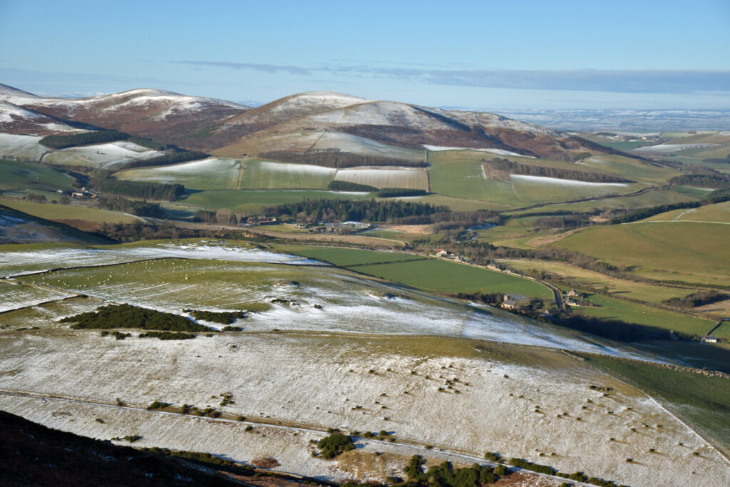
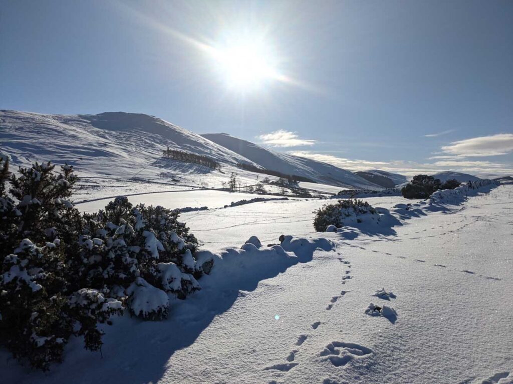
My first encounter with the Wall was a birdseye view (Fig 1), seen through the eyes of a raven familiar (don’t worry about the backstory, just go with it). This birdeye view provides a very impressive sense of scale of the Wall – it takes ages to fly to it (as you are forced in the game to travel from the South of England) and compared to all the other settlements and locations in the game, it is simply huge! The aerial view also gives you a sense of landscape, and from the correct altitude, you can see the Wall as it leads from the low-lying coast up into snow-covered wintry hills. 

Fig 1: Birdeye view of Hadrian's Wall

But you can also explore Hadrian’s Wall on the ground. The game actually has a major quest that forces you to the Wall, but we’ll just set that aside for the moment. Whether you approach the Wall on your own two feet, or on the hooves of your trusty steed, the Wall is an imposing monument. It winds its way across the ancient kingdom of Northumbria (in the game, reduced Eurvicscire), and let me tell you, it can be slow-going walking uphill in a virtual blizzard!

So, how does the virtual Wall look, compared to the real deal? Visually, it looks great and is quite interesting (Fig 2). In terms of historical accuracy, however, it will definitely set off sensitive pedantometers. Before we get too catty, though, it is worth remembering that there is no location where Hadrian’s Wall survives to its full height, nor do we have any accurate historical depictions of the Wall. Typically, we have less than 2 meters of standing monument, and in some exceptional cases that extends to 3-3.5m. This is a gentle reminder that there is A LOT that we do not know about Hadrian’s Wall.

Fig 2: South face of Hadrian's Wall

But let’s explore the virtual Wall, and consider how insightful and helpful Ubisoft’s work has been.

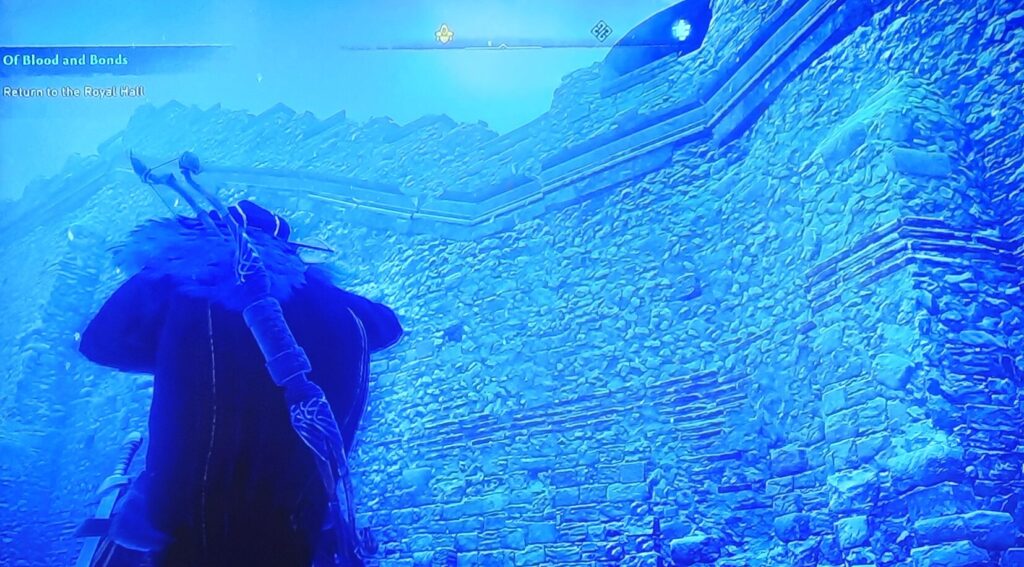
Staring with the curtain itself, the virtual Wall is certainly made of stone like the real Wall, but the virtual Wall has a wider range of materials and sizes than seen on the real Wall. If you look at Fig 2, you can see Eivor standing near the south face of the virtual Wall at ground level. The lowest courses display reasonably accurate-sized blocks that have been roughly shaped and course. Looking up the face of the curtain, though, you see smaller unshaped stones that appear to be rubble, held in place with variably weathered mortar. There are also bonding course of red tile, and buttresses to reinforce and support the height of the curtain. Near its top, a nice sandstone string course remains in situ, occasionally damaged. Atop the virtual Wall, there is a wallwalk with a crenelated parapet on the north side (Fig 3). In terms of a broader practice of Roman architecture, the virtual Wall is reasonably accurate. However, with real Wall there is no evidence for tile-bonding courses or buttresses. Rubble blocks were only used for the core of the Wall, which was otherwise faces with roughly dressed sandstone blocks. As for the wallwalk, this is something that is debated amongst Hadrian’s Wall scholars, and for which there is no direct evidence (it is all circumstantial). There is, however, evidence of stone slabs with bevelled edges that are believed to have formed a string course near the top of the real Wall curtain.

Fig 3: Wall walk

A turret can be seen in Figure 4, as approached from the south east. From this view, the turret itself is a very good digital reconstruction of one potential version of what a real Wall turret would have looked like, based on examples carved in Trajan’s Column (erected and still standing in Rome). The oddity in this image, however, is the staircase. Turrets along Hadrian’s Wall were accessed through a door in the southern wall set at ground-level. Also, if you move to the front of the turret, it has a semi-circular front (Fig 5). These sort of D-shaped towers are found at Roman military sites, but not until the later 3rd and 4th centuries AD, at least 150 years after Hadrian’s Wall was originally built.

Fig 4: South face of a turret

Fig 5: Front of a turret

Some explorers of the virtual Wall will also be disappointed to learn that there are no milecastles. There are, however, three fort sites, and a small number of slightly larger octagonal towers and considerably larger tower complexes (more akin to a fortified tower of the 12th-13th centuries).

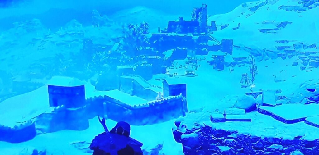
The forts are those at Newcastle, Housesteads, and Carvoran. Housesteads is a named location, and Carvoran is called Magnis in the game (close to its Roman name of Magna). Both the forts at Newcastle and Housesteads are largely covered in deep snow drifts and cannot be explored fully, though climbing along rooftops provides some elevated views of the forts (Fig 6). A few buildings can be partially explored, and the north gate of Housesteads projects out of the snow (Fig 7).

Fig 6: Inside of snowy Housesteads fort

Fig 7: North gate of Housesteads

The fortress at Magnis is a site of the storyline in the game, and it is more fully modelled. In truth, it is not a site anyone familiar with Carvoran would recognise, or any fort of Hadrian’s Wall. Magnis is far larger and with considerably taller buildings than a Hadrian’s Wall fort would have had (Fig 8). It also lies at the western end of the playable area of the game, and therefore defines the western end of the virtual Wall in the game.

Fig 8: Magnis fortress

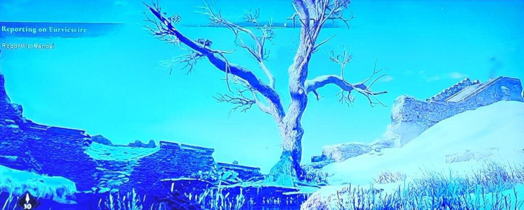
While it was not possible to replicate every location along Hadrian’s Wall in the game, visitors will still recognise Sycamore Gap, the tree bare of leaves in this winter landscape (Fig 9).

Fig 9: Sycamore Gap

With these aspects in mind, it is clear that the virtual Wall in Assassin’s Creed is not a very accurate structural reconstruction of Hadrian’s Wall. It is a fictionalised monument, inspired by the original, but modified for the purposes of gameplay.

Now, some might decry such digital fantasies, but consider the alternative. Hadrian’s Wall, as it appears now and as it might reasonably be reconstructed, is actually a surprising boring monument, visually speaking. Don’t believe me? Try making a model of Hadrian’s Wall out of Lego – it does not make for the most visually engaging build…

The virtual Wall in Assassin’s Creed is a super-charged version of Hadrian’s Wall. While it retains the likely original height, it is thicker, and the surface rendering of different stones and tile bonding courses creates a more visually engaging monument. Furthermore, the artful fashion in which the virtual Wall is cracked, fractures, and in some places collapsed, lends to the sense of lost empire.

Ironically, the might of Rome and the loss of a world-spanning empire is felt throughout the game, not just via Hadrian’s Wall but through all the ruinous Roman sites found in 9th-century England.

by Rob Collins

Just Breathe

Figure 1: Westnewton, where the College Burn meets the River Bowmont, together forming the River Glen

The route from my house which follows the road to Hethpool and the College Valley is a favourite and regular running route for me.  From Kirknewton the road runs past the village hall and St Gregory’s, the (originally) 12th century parish church with its famous kilted-magi. Beyond this there are flat, flood-plain fields bounded by steep hills, and the old railway-station houses. Shortly before Westnewton the road crosses the College Burn, just upstream of its confluence with the River Bowmont, the combined rivers flowing on down Glendale as the River Glen.

In Westnewton the road to the College Valley turns off the main road and past the large Edwardian house of the Kirknewton Estate now owned by Simon Douglas-Hume (an interesting merger of two reiving family names). To reach the College Valley the road takes a detour up around the Bell (a hill!) west of the College Burn before reaching a saddle at 500 foot and then dropping down to Hethpool and into the College Valley. This glacial valley, one of the most beautiful in the Cheviots, runs right the way up to the Border Ridge between the Cheviot itself and the Schil and offers the best route onto the Cheviot via Hen Hole.

On the way back I like to push myself, after the long run downhill in the College Valley, to a fast run up the saddle by the Bell before easing into the final run-out back down to Westnewton and then home. It always strikes me, when I get to the top of the saddle having pushed hard to that point, that as I relax into the downhill that my breathing continues to get harder. There is a time-lag between reducing the effort put into running and my breathing rate, maybe a consequence of an oxygen debt built up, with the body requiring time to adjust to the new level of effort.

Figure 2: running in the Cheviots

Figure 3: The sun 8 minutes before this picture was taken

Change in breathing-rate is one of many processes which have an associated time lag. The slow increase in the sea’s temperature lags behind the warmth we feel in the air as the sun’s radiance warms through Spring. The sun that we look at (through dark glasses) is the sun of 8 minutes ago, as even at the speed of light it takes this long to travel the 193 million miles in between.

The operation of our planet’s geological, biological and atmospheric processes and the interaction between them contain several examples of this type of lag.

Perhaps the earliest and most protracted of these was the first development of oxygen in the atmosphere, way back in the Archaean. This event was not only crucial to my very existence, but also my ability to run up hills, with the energy released by oxidation powering my fast metabolism as well as that of all multi-celled organisms and most single-celled organisms. This time lag is between the evolution of oxygenating bacteria and the oxygen they create arriving in the atmosphere. Some 3.5 billion years ago (that’s one thousand times older than the Carboniferous rocks which underpin Hadrian’s Wall) in the early Archaean the atmosphere had an unquantified mix of nitrogen, carbon dioxide, methane and ammonia. What we do know is that there was no oxygen in this atmosphere, as iron on the surface didn’t rust.

Figure 5: a modern cyanobacteria

What was needed was something that would break out the oxygen contained in atmosphere’s CO2. This something evolved early in the Archaean as cyanobacteria, which could use iron and CO2 mixed with the energy of sunlight to grow their bodies. There were, however, other blocks in the pathway to releasing oxygen into the atmosphere. The first was that the earliest cyanobacteria didn’t make free oxygen, they made iron oxide instead. This, however, was not a problem, as the second block was an oceanic addiction to iron, which dissolves readily in seawater in the absence of oxygen. This mass of dissolved sea iron meant that any oxygen created simply reacted with the dissolved iron, which promptly precipitated as iron oxide and sank to the bottom. Our early cyanobacteria, by making iron oxide as a by-product, were steadily mopping up this dissolved iron.

Figure 4: an outcrop of the Banded Iron Formation in Australia

By the time cyanobacteria evolved to produce free oxygen later in the Archaean, there was less dissolved iron to steal this oxygen. By the end of the Archaean and moving into the Proterozoic Era 2.5 billion years ago, free oxygen arrived in the atmosphere and the surface of the earth started to rust. This was an unimaginably slow process, taking a billion years, 3 times longer than the length of time between our Carboniferous rocks and the present.

The consequences were immense, providing the starting point for the evolution of life as we know it as well as depositing massive quantities of iron. These deposits consist of finely banded layers of iron oxide (haematite) and chert and is known as the banded iron formation. This is by far the most important source of iron used by homo sapiens.     

Oxygen also features in a delayed response nearer to home and nearer in time, in which evolution and geology feature once more. This is the time lag between the arrival of plants on the land surface and radical changes in atmospheric O2 and CO2 during the Carboniferous Period.

Figure 6: Artist’s impression of Arthropleura

Imagine finding a centipede under a rock. Now imagine that centipede is over 2m long and half a metre wide. This is what happened to a Cambridge research student a few years ago, on a walk along the shore at Howick on the Northumberland coast. Admittedly the creature was a long time dead, having been preserved in one of the silty sandstones of the Carboniferous period which crop out on the coast here. Nonetheless it was spectacular find, being the largest specimen of a creature named Arthropleura which has ever been found. This gigantism is a feature of many groups of Carboniferous animals. It is particularly surprising to find such a large arthropod which group of animals respires by diffusion through its skin. This is one line of argument indicating that during parts of the Carboniferous period the levels of oxygen in the atmosphere exceeded 30%, compared to current levels of 21%. With that amount of oxygen my run up the College Valley would have been at a solid road-runner pace – meep meep!

The size of the Howick Arthropleura specimen, which comes from the middle Carboniferous, has been compared to that of specimens from various times earlier in the Carboniferous. This shows a progressive increase in the size of the animals which is thought to relate to the progressive rise in oxygen levels in the atmosphere. At the same time, we know that the levels of CO2 in the atmosphere decreased, and after a lag in time, the global climate also became cooler. This cooling has strong evidence from glacial deposits – tillites – which show that ice-caps formed during this period. Why was the atmosphere changing? It seems that once more we have evolution to thank, but this time in plants.

Figure 7: Size increase in Arthropleura from Davies etal 2021

Plants had colonized the land surface many millions of years before the Carboniferous. Fossil liverworts have been found in the late Silurian period (at 425 million years old) and recent research using DNA suggests that there may well have been land plants some 100 million years earlier, during the Cambrian Period. No doubt these plants started to contribute to the removal of CO2 and the generation of O2 as they grew and respired.  So why the long delay before the effect is seen in the Carboniferous Period, both in the atmosphere and in the climate? Three possible reasons stand out.

Figure 8: reconstruction of a coal swamp

The first is the presence of lignin, which had evolved by the beginning of the Carboniferous Period. Lignin decays more slowly than softer plant tissue. Additionally, fungi which now break down lignin may not have evolved in the Carboniferous Period. This meant that at that this time more dead wood was taken out of circulation through burial by sediment rather than by oxidisation and consequent release of CO2 back into the atmosphere.

The second reason follows in part from the presence of lignin. During the Carboniferous significantly more of the land surface became colonised by plants in terms of the land surface and ecological niches covered as well as by the sheer size of the plants. The giant lycopods which were one of the major plant types of the Carboniferous not only grew to many tens of metres in height but also had a phenomenal growth rate. Together this means that the volume of carbon-rich plant material available for burial vastly increased at this time.

The final reason is linked to the changes brought about in the atmosphere, in particular the very high levels of oxygen. The progressively more devastating wildfires seen in California and Australia are awe-inspiring and terrifying to watch. However, this would have been a whole lot worse and much more frequent with an oxygen-rich atmosphere. The Carboniferous forests were frequently on fire which meant that large amounts of charcoal were produced. Charcoal decomposes much more slowly than wood and other plant tissues and more of it gets buried. So, whilst the fires themselves turned oxygen and trees back into CO2 the charcoal meant that much more of the trees’ carbon was buried and taken out of the carbon cycle (at least until the present day!).

Figure 9: A wildfire in Montana, USA

The ice caps that formed during the Carboniferous Period disappeared towards the end of the period over 300 million years ago. They didn’t return until about 2.5 million years ago. There is much evidence we can glean from rocks and fossils of the Carboniferous period regarding climate change.  However, the data available on climate change from our recent past is much more detailed. Now and in our recent history we have been measuring changes in climate around the world and the impact this had on natural processes. To go further back there is a geological record forming, for example, in the form of layers of sediment at the bottom of lakes and in the sea; much can be learned from these. There is also another more ephemeral (in geological timescales) source of information, which is ice. Snow is seasonal and as it falls, snow on snow, in the Arctic and Antarctic areas and slowly compacts forming annual layers which can be read back like the rings of a tree. Within the ice, bubbles of the atmosphere become trapped so that it is possible to see changes in CO2 levels along with other atmospheric components. There is a lag in this process too, as it takes many years for the snow to compact sufficiently that the air bubbles are sealed in. The date the snow is laid down and the age of the atmosphere it eventually traps are different by a few hundred years.

Figure 11: This month’s mystery rock, an ice core from the Arctic

Not only is it possible to analyse historic changes in atmosphere, but analysis of the oxygen and hydrogen isotopes in the ice also tell of the temperature when the ice formed. Between these analyses it is therefore possible to build up a detailed picture of the relationship between temperature and carbon dioxide. This month’s mystery rock is one of many ice-cores recovered from the Arctic and used for this purpose. Analyses of these ice-cores reveals a lock-step relationship between temperature and CO2; when temperature is higher so is CO2 and vice versa.

Figure 10: the relationship between atmospheric CO2 and temperature.

There is however another time-lag here. When the temperature rises, there is a delay before CO2 levels start to rise. It is a mantra of scientists that correlation doesn’t necessarily mean causation, and some people use this stick to discredit the idea of manmade climate change; if CO2 rises after temperature increase, then is can’t be the cause of that temperature change. However, the reality is much more complex.

There is no doubt that an increase in CO2 causes global warming as it is a physical property of the gas, but there is another cause for changes in global temperature. This is to do with the amount heat we receive from the sun which varies over time. The earth’s rotation around the sun is not fixed and constant but wobbles ever so slowly and in several different ways. Firstly, the earth’s orbit is an ellipse, and not a circle, and furthermore the shape of that ellipse (the orbital obliquity) changes over time between something more circular and something more elliptical. Secondly the earth’s axis is tilted, a fact which gives us our seasons, and both the amount of tilt (axial tilt) and its orientation towards the sun change over time (axial precession). Each of these wobbles mean that the amount of heat the earth captures from the sun (its insolation) changes progressively and predictably over time. The sums to make those predictions were first carried out, meticulously and laboriously in a pre-computer age, by a Serbian mathematician Milutin Milankovitch. These Milankovitch cycles as they have become known correlate precisely with changes in global temperature. It now seems clear that increases in global temperature are initiated by the changes in insolation described by the Milankovitch cycles.  As the temperature rises, this causes more CO2 to be generated which then significantly amplifies the initial increase in temperature.

Figure 12: Milutin Milankovtich

This brings us back to the present day, cooling down in my garden with a large glass of elder cordial in hand contemplating what happens next. What can be predicted of where global climate is heading from our knowledge of Milankovitch Cycles and the detailed record of our immediate past which the ice cores give us? Even with all of this data it seems that this is hard to predict. It is likely that without manmade CO2 there will come a point in the next 10 to 40 thousand years that the global climate cools. However, that manmade CO2 is there in quantities not seen for over 2.5 million years.  

Figure 14: Vindolanda tablet; letter from Octavius to Candidus

At that time there were no icecaps, and the sea level was over 100 feet higher than it is now. Our contribution to atmospheric CO2 continues to grow in volume.

The peat at Vindolanda and other locations along the Wall is drying out owing to the dryer warmer climate being experienced in this part of the world, a likely in consequence of manmade climate change. It may well be that the delicate leather and wood artefacts so beautifully preserved by the peat will start to oxidise as the drying continues and deny us the wonder and information they bring. Just one small consequence of the direction of travel we see emerging.

At this point I wonder at mankind’s collective action in the time-lag between continuing to create atmospheric CO2 and its likely consequences. It seems rather like the time-lag in the ever-outwitted Wylie Coyote as the slow grinding of his mental cogwheels finally give him the dawning realisation that he is running in thin air, shortly before plummeting into the canyon below.

Figure 13: Trees felled by Storm Arwen at Old Bewick, a taste of things to come?

Attributions

The idea for this blog was inspired by a reading of “The Goldilocks Planet” by Jan Zalasiewicz and Mark Williams. For much more detail about some of the ideas presented here (and somewhat simplified) this is an excellent and readable book.

Ice Core: This photograph shows a section of the GISP2 ice core from 1837-1838 meters in which annual layers are clearly visible. The appearance of layers results from differences in the size of snow crystals deposited in winter versus summer and resulting variations in the abundance and size of air bubbles trapped in the ice. Counting such layers has been used (in combination with other techniques) to reliably determine the age of the ice. This ice was formed ~16250 years ago during the final stages of the last ice age and approximately 38 years are represented here. By analyzing the ice and the gases trapped within, scientists are able to learn about past climate conditions. Soerfm, CC BY-SA 4.0 <https://creativecommons.org/licenses/by-sa/4.0>, via Wikimedia Commons

The sun: NASA, Public domain, via Wikimedia Commons: This photograph of the Sun, taken on December 19, 1973, during the third and final manned Skylab mission, shows one of the most spectacular solar prominences ever recorded, spanning more than 588,000 kilometers (365,000 miles) across the solar surface. The loop prominence gives the distinct impression of a twisted sheet of gas in the process of unwinding itself. In this photograph the solar poles are distinguished by a relative absence of supergranulation network, and a much darker tone than the central portions of the disk. Several active regions are seen on the eastern side of the disk. The photograph was taken in the light of ionized helium by the extreme ultraviolet spectroheliograph instrument of the U.S. Naval Research Laboratory.

Cyanobacteria: TEM image of ”Prochlorococcus marinus”, a globally significant marine cyanobacterium : Luke Thompson from Chisholm Lab and Nikki Watson from Whitehead, MIT, CC0, via Wikimedia Commons.

Banded Iron Formation: Banded Iron Formation at the Fortescue Falls, Karijini, Australia: Graeme Churchard from Bristol, UK, CC BY 2.0 <https://creativecommons.org/licenses/by/2.0>, via Wikimedia Commons

Arthropleura: Artist’s impression of Arthropleura (which has some anatomical inaccuracies, but gives a good idea of scale). Tim Bertelink, CC BY-SA 4.0 <https://creativecommons.org/licenses/by-sa/4.0>, via Wikimedia Commons

Arthropleura size comparison: from Davies etal 2021, Journal of Geological Science. The Largest Arthropod in Earth History.

Wildfire: Elk in the Bitterroot River at Sula, Montana, during a fire in the year 2000. Photo by John McColgan, fire behaviour analyst with the BLM’s Alaska Fire Service: John McColgan – Edited by Fir0002, Public domain, via Wikimedia Commons

Graph of CO2 v Temperature: This shows historical carbon dioxide (right axis) and reconstructed temperature (as a difference from the mean temperature for the last 100 years) records based on Antarctic ice cores, providing data for the last 800,000 years. Leland McInnes at the English-language Wikipedia, CC BY-SA 3.0 <http://creativecommons.org/licenses/by-sa/3.0/>, via Wikimedia Commons

Milutin Milanković: Unknown author, Public domain, via Wikimedia Commons

Vindolanda letters: Roman writing tablet from the Vindolanda Roman fort of Hadrian’s Wall, in Northumberland (1st-2nd century AD). Tablet 343: Letter from Octavius to Candidus concerning supplies of wheat, hides and sinews. British Museum (London): British Museum, CC BY-SA 3.0 <https://creativecommons.org/licenses/by-sa/3.0>, via Wikimedia Commons

Figure 6. (a)-(e) Geological epochs and earth atmospheric temperature (˚C, ˚F vs. 1960-1990 avg.) (Bredenberg, 2012).

Figure 7. CO2 and temperature over past 420,000 years (Watts & Pacnik, 2012).

A Foot in the Slime

Waves crasing on rocks under bright blue skies
Figure 1: Whitley Bay - the stripy sandstones

If you had asked me three years ago about open water swimming, I would probably have given you a luke-warm response. Having been persuaded by my partner Rachael to give it a go I can conclusively say that luke-warm is not a suitable response to open water swimming. The North Sea is categorically Baltic in the winter months and swimming at these times comes with a generous cake-slice of insanity, albeit mixed in with a vibrant sense of being alive. One of our favoured spots for swimming is in Whitley Bay from the Panama Swimming Club clubhouse.

The beach here is sandy, but with a variable sized collection of stones strewn across the surface and a reef of beautifully striped sandstone pointing from the Spanish City out towards St Mary’s lighthouse. As an unreconstructed geologist I can’t help scrutinizing the pebbles on the beach as I trepidate towards the freezing water. For the most part these are a collection of water-worn sandstones (some with beautiful stripey patterns) and limestones not infrequently spotted with the remains of the communal coral Siphonodendron. On occasion there are small brown, flat slabs of hard sandy limestone to be found, filled with cream-coloured smiles. These are the cross-section of fossil bivalves preserved in multitudes within these stones. It is one of these stones that features as mystery rock number 23 for the WallCAP Newsletter.

Figure 2: Mystery Rock 23

Figure 3: The Low Main Mussel Band exposed at Whitley Bay

A visit to the beach at Whitley Bay in early March 2021 would not have been the time to go for a swim. A storm the previous weekend had almost completely stripped the beach of its sand, leaving a wasteland of boulders and pebbles. It also exposed more layers of bedrock than the regularly visible reefs of stripy sandstone. Amongst these newly exposed layers was the source of the fossil smiles, a layer no more than a few inches thick just above the stripy sandstones and containing thousands of these fossils.

This layer of rock is the Low Main Mussel Band, which lies just above the Low Main coal seam after which it is named. The mussels, a type of bivalve, are of three species, Carbonicola (which used to be called Anthracosia), Anthrocanaia and Naidites. As usual with fossils, their presence helps unravel what was happening when these layers of rock were being laid down.  In addition, this type of shelly layer is found scattered through geography and time in the sequence of late Carboniferous rocks (the Pennine Coal Measures Formation) of Tyneside.  So, what are these fossils and what do they tell us?

Figure 4: Detail of the Low Main Mussel Band

Figure 6: Swan Mussel - Anodonta cygnea

In the very dim and distant past, I used to belong to the 1st Central scout group which met in a hut adjacent to the underground sidings behind Morden Station in south London. In this pack I rose to the dizzy heights of being a sixer, a role, which brought variable results. At a scout camp competition where we were to show off our camping and woodsman skills, our “six” successfully dug a magnificent latrine. This was discovered inadvertently during the night by one of the judges who fell into it. What we learned was that the middle of a footpath is not a good place for a lat-pit (and we didn’t do well in the competition). On a brighter and better occasion, we camped at a Longridge on the River-Thames near Marlow, a campsite which mercifully had flushing toilets. One of the main purposes of this camp was to learn how to canoe. Learning how to canoe, it seems, involves a great deal of falling out of canoes and a great deal of close up familiarity with the river. One of the things I discovered through multiple visits into the murk of the Thames water was that my feet on the riverbed squelched into layers of silty mud. To my surprise, within this mud lived some magnificent bivalves several inches long and with beautiful glossy green shells. These were swan mussels (Anodonta cygnea). I recollect my surprise at finding bivalves in a river rather than in what I thought of as their natural habitat, which is in the sea. It is the case that the modern landscape of sea-shells is dominated by the phylum of Mollusca either in the form of bivalves (cockles, mussels, clams and the like) or as gastropods (winkles, whelks, limpets and the like). There was, however, a different story to be told of the Carboniferous bivalves, which finally returns us to the question I asked a paragraph back.

Figure 5: Cockles and Mussels - modern bivalves

The Carboniferous bivalves to be found in the Low Main Mussel Band are, like the River Thames’ swan mussels an indicator of fresh or brackish water. This marks a significant change from the swamp-land conditions in which the coal of the Main Coal seam was forming and may relate to a rise in sea-level. These mussel bands, of which there are many in the Pennine Coal Measures Formation, are surprisingly continuous over many kilometres. This makes them a useful signpost, not only of the geological conditions in which they were laid down, but also of where you are in the rock sequence and in time. A coal miner coming across the Low Main Mussel Band would know that they were immediately above the Low Main Coal seam. Each of the other mussel bands scattered through the Pennine Coal Measures Formation has different types of bivalves (and other fossils) in them. This was not just down to the mussel beds forming in different environments (which favoured one or other type of creature) but also a result of evolutionary change. In the time interval between the formation of different mussel bands, some creatures had become extinct and new creatures had evolved.

Figure 7: Brachiopod anatomy

Figure 8: Spirifer striatus

So what happens if we make the comparison between a river or estuarine environment and a marine environment in the Carboniferous as we did for the modern day? It reveals that the dominant species of sea-shell in the Carboniferous were not molluscs of any stripe, but another group of creatures with two shells, the brachiopods. The Brachiopoda form a phylum in their own right completely separate from the Mollusca. The name brachiopod comes from the ancient Greek and means arm-foot. The “foot” is the most obvious part of a live brachiopod, with a muscular column called a pedicle, which extends from the bottom (ventral or pedicle) valve of the animal. Brachiopods use this foot to secure themselves to the sea floor. The “arm” is found on the inside of the shell as part of the upper (ventral or brachial) valve. It is not an arm in any mammalian sense, rather a support structure for a part of the animals feeding apparatus called a lophophore, a whiskery, horseshoe shaped structure. These brachial structures, which support the lophophore vary in their complexity. For example, in the brachiopod family of Spirifers (common in the Carboniferous) they form elegant spiral structures which give the Spirifers their name.

Figure 9: A Roman oil lamp and a terebratulid brachiopod

Brachiopods are also known as lamp shells. This comes from the similarity in shape between the brachiopod family of Terebratulids and Roman oil lamps.  The name Terebratulid comes from the Latin for hole borer (terebra) – the reason for the derivation is not clear, but maybe because the small circular hole in the shell, through which the pedicle would have emerged and

looks like it has been drilled, is so clearly seen in these animals. The Terebratulids are also one of a handful of brachiopod orders that survived the largest mass extinction event, known as the Great Dying, at the end of the Permian period 252 million years ago. This event also marked the fulcrum around which the balance of ecological power

Figure 10: Lingula (modern) and Lingulella (ancient - Cambrian)

between the molluscan bivalves and the brachiopods hinged. The brachiopods are remarkable in their persistence through geological time. There is one species, Lingula, which may be found in brackish estuarine sediments (hostile to many organisms) and there is a remarkably similar (although evolutionary distinct) burrowing brachiopods which is preserved in rocks of Cambrian age (circa 550Ma). However, the rich list of brachiopod species and the range of ecological niches they filled during the Palaeozoic era (including the Carboniferous period), has now been usurped and almost entirely filled by molluscan bivalves. Next time I visit Whitley Bay for a bracing dip, it will be the limpets and cockles (molluscs all) I will share the swim with, whilst I contemplate the brackish waters of the Low Main Mussel Band and their ancient cousins.  

Figure 11: Whitley Bay at sundown

Attributions

Swan Mussel: Anodonta cygnea. Jakob Bergengren, CC BY-SA 3.0 <https://creativecommons.org/licenses/by-sa/3.0>, via Wikimedia Commons

Mussels: Derrick Mercer, CC BY-SA 2.0 <https://creativecommons.org/licenses/by-sa/2.0>, via Wikimedia Commons

Cockles: Cardium indicum Lamarck, 1819 – hians cockle. James St. John, CC BY 2.0 <https://creativecommons.org/licenses/by/2.0>, via Wikimedia Commons

Spirifer: Two specimens of Spirifer striatus (named as Spirifera striata in the original). From Plate XXXI of Monograph of British Fossil Brachiopoda Volume 4 Part 3.

Roman lamp: Ancient Roman oil lamp in D. Diogo de Sousa Museum, Braga, Portugal.. Joseolgon, CC BY-SA 4.0 <https://creativecommons.org/licenses/by-sa/4.0>, via Wikimedia Commons

Terebratulid: Terebratulid brachiopod from the Campanian (Upper Cretaceous) of southwestern France. wilson44691, CC0, via Wikimedia Commons

Lingula: Lingula anatina shell found in the Mediterranean Sea, in a laboratory of practices of the Faculty of Sciences of the University of Corunna. I, Drow male, CC BY-SA 3.0 <https://creativecommons.org/licenses/by-sa/3.0>, via Wikimedia Commons

Lingulella: Lingulella lingulaeformis Mickwitz, Leptembolon lingulaeformis (Mickwitz, 1896). Estonian Museum of Natural History, CC BY-SA 4.0 <https://creativecommons.org/licenses/by-sa/4.0>, via Wikimedia Commons


A Reef in Time

My nose was almost touching the shiny grey-white undulating slab of stone that was slick with moisture. My head was similarly close to the slab of stone above me, though I couldn’t see what it looked like. My elbows and forearms were inching me forward combined with whatever purchase I could get from my toes. In front of me my right hand held a carbide lamp with its silent elegant feather of acetylene flame guiding me forwards. This was me in my first year of doctoral research having decided I wanted something interesting and exciting to do. The Imperial College Caving Club provided this, heading out to the Brecon Beacons in an old ford car for a weekend of underground adrenaline. I can think of no other occasion when I was so closely surrounded by lime in different forms, though a caving trip to the Mendips as part of a management training exercise and trips to the disused chalk quarries above the Silent Pool in Surrey (coming home caked in chalk), come a close second.

A young geologist wearing a bright yellow waterproof suit and an orange hardhat with a headlamp leans against the wall of a dim cave.
Figure 1: a younger version of a community geologist in a cave in the Mendips

Figure 2: a carbide lamp

The carbide lamp was an elegant testament to the many industrial uses that lime is a part of. The calcium carbide which was one part of the fuel which powered the light is a product of calcium oxide and coke heated to high temperatures in an electric arc furnace. The calcium oxide in turn is a product of limestone which has been heated in a lime kiln to over 800C, breaking down the calcium carbonate (which the limestone is composed of) into calcium oxide and CO2. The other part of the lamp’s fuel is water, which drips onto the powdered calcium carbide at the base of the lamp, reacting with it to produce acetylene. The acetylene burns with a small, pointed flame of bright light, perfect for caving. The lamp is literally in its element in a limestone cave and is still used by some cavers as their preferred source of light.

Carbide lamps have also been used by many generations of miners albeit the naked flame was a hazard in coal mines. This led to its replacement in this setting by the Davy lamp, with its gauze cover reducing the risk of igniting the coal gas.

The chemistry of calcium carbonate has not just been exploited by industrial man but also by a remarkable range of creatures throughout the history of life on earth. One of the earliest pieces of evidence for life are laminae of calcium carbonate in mounds about a metre across which resemble structures, called stromatolites. These are the product of microbial mats produced by cyanobacteria and growing in shallow water where they trap fine lime-rich sediment. The oldest of these are some 3.5 billion years old in the early Archaean eon and discovered in sandstone from western Australia.

Figure 3: ancient stromatolite from Strelly Pool Chert, Western Australia.

Small, dark rounded mounds of mineral
Figure 4: modern stromatolite reef, Shark Bay, Australia.

Stromatolites reached the peak of their diversity in the late Proterozoic eon though they can still be seen today. These are not only the earliest life forms but also show the way that organisms started use lime as a way of protecting themselves and in doing so beginning to form reef like structures.  

The journey from here to the astonishing diversity of life on a modern coral reef is a long one with periods of progressive ecological diversification and colonisation, but with some major setbacks too. By the Devonian period, some of the largest reefs that ever occurred on earth had developed.

These reefs were dominated by stromatoporid sponges, along with tabulate and rugose corals, a markedly different mix of animals from our modern reefs. Not only were there different ratios of reef-forming families, with sponges more common than corals, but also these Devonian sponge and coral orders are all now extinct.

Towards the close of the Devonian period, there was an extinction event, the fourth largest of the Phanerozoic (the current geological eon). This extinction event, thought to be caused by climatic cooling – a precursor of the glacial conditions which fluctuated throughout much of the Carboniferous period – wiped out the stromatoporoid corals and severely impacted both the tabulate and rugose coral families.  

Figure 5: stromatoporoid sponges from the Keyser Formation, Pennsylvania, USA

A chart showing the changes to coral groups over time
Figure 6: diversity of the main coral groups in the Phanerozoic Eon

It wasn’t until the Triassic period, with the cold global climate of the Carboniferous long in the past that reef building on the scale of the Devonian returned. This also post-dated the “great dying” at the end of the Permian Period, the largest mass extinction the earth has seen, when life on earth was nearly wiped out. This extinction event finally finished off the tabulate and rugose corals and, in the Triassic, these old-order corals were replaced by the modern sclerectinian corals.  These corals had a lighter structure than the rugose and tabulate corals and were made of aragonite (a polymorph of calcium carbonate) rather than calcite (the other polymorph of calcium carbonate). Sclerectinian corals are also know for their symbiosis with the photosynthesising algae, the Zooxanthellae. This partnership gives the corals an advantage in fixing lime from atmospheric CO2, and it may be that this collaboration gave these corals an edge in colonising and diversifying throughout the world.

It remains an article of debate as to whether the older rugose and tabulate families of corals had this ability. This advantage to growth had its downsides though. When it came to mass extinction events, the zooxanthellate corals were at a disadvantage, constrained as they were to shallow water and more vulnerable to changes in temperature and ocean acidification. This was borne out in the mass extinction at the end of the Cretaceous period where the asteroid impact at Chicxulub in Mexico, not only wiped out the dinosaurs but many other families. The corals that survived this event tended to be deeper water, non-zooxanthellate organisms. You can’t hold a good idea down though, and following this catastrophe, the symbiotic relationship was re-established independently in several coral families.

Figure 7: Microscopic Zooxanthellae aka Symbiodinium found in corals

Brightly coloured, spikey colar under the water
Figure 8: Modern sclerectinian corals on the Flynn Reef near Cairns in Australia.

The diversification of species of reef building animals to fill a wider range of ecological niches and larger areas of the sea-bed is not just controlled by evolution and natural disaster. There is wider rhythm to fluctuations in diversity and range related to changes in climate. One of the consequences of the change from a glaciated world to a hotter global climate with no polar ice caps is that higher sea levels flood continental shelves to create more extended shallow marine environments. As a result, hotter worlds such as the Silurian to mid-Devonian or the Triassic to Cretaceous had much larger habitats in which corals and other reef forming organisms could thrive. It may be that during the Carboniferous period, much of which sported polar ice caps, the consequent low sea levels and restricted shallow sea environments contributed to the slower development of reef habitats.

The Carboniferous period, however, was not without its reefs and was categorically not without limestones which formed from the remains of calcifying animals. Without these limestones the Romans would not have had a source for making lime with which to help stick the Wall together. The remains of reef like structures made up of rugose corals can be seen, for example, on the Northumberland coast. It is during this period that the thick shelled productid brachiopods become common a well as the elegant plant-like crinoids. These three animals are the dominant calcifying creatures of the Carboniferous, and their fossils are the ones you are most likely to find if you happen to come across a limestone outcrop when exploring the Wall.

Figure 9: large rugose coral in life position near Spittal on the Northumberland coast

Figure 10: mystery rock 22, a limestone pavement at Beadnell on the Northumberland Coast, where the limestone joints have been enlarged by water preferentially dissolving the cracks.

I am certain that there would have been some of these fossils under my nose in that cave in the Brecon Beacons, however my mind was otherwise occupied at that moment. The steady drip of the water into the calcium carbide of my lamp making the acetylene to light my way forward seemed an appropriate reminder of the slow work of water in the cave I was crawling though. Limestone is soluble in water, particularly when acidified by dissolving CO2. As the limestone dissolves it produces some beautiful landforms, including the limestone pavement which was Mystery Rock number 22 for the WallCAP newsletter last month. It also completes the cycle started by the corals and crinoids and brachiopods fixing the calcium and carbonate ions into their shells, and now being dissolved and returned via the river to the sea.

It is also a reminder, as levels of anthropogenic CO2 continue to rise, that rising global sea temperatures and an acidifying ocean make our extraordinarily diverse, complex and beautiful reefs vulnerable. What will be the role of reefs be in the future, as we move into what is now commonly referred to as the Anthropocene?

Figure 11: A healthy reef (Lodestone Reef, Queensland, Australia) and one bleached by high ocean temperatures (Island of Reunion).

Attributions

Stromatolite: Stage : Paleoarchean from 3 600 to 3 200 Ma (million years ago). Locality: Strelley Pool Chert (SPC) (Pilbara Craton) – Western Australia. By Didier Descouens – Own work, CC BY-SA 4.0, https://commons.wikimedia.org/w/index.php?curid=15944367

Modern stromatolite: Stromatolites growing in Hamelin Pool Marine Nature Reserve, Shark Bay in Western Australia. Paul Harrison, CC BY-SA 3.0 <http://creativecommons.org/licenses/by-sa/3.0/>, via Wikimedia Commons

Stromatoporid Sponge: Jstuby at English Wikipedia, Public domain, via Wikimedia Commons.  Stromatoporoids in the Silurian-Devonian Keyser Formation, Old Eldorado Quarry, in Blair County, Pennsylvania.

Corals through time: https://www.bgs.ac.uk/discovering-geology/fossils-and-geological-time/corals/

Modern corals: By Toby Hudson – Own work, CC BY-SA 3.0, https://commons.wikimedia.org/w/index.php?curid=11137678. A variety of corals form an outcrop on Flynn Reef, part of the Great Barrier Reef near Cairns, Queensland, Australia.

Zooxanthellae: By Todd C. LaJeunesse – flickr, CC BY-SA 2.0, https://commons.wikimedia.org/w/index.php?curid=79980176 Symbiodinium, colloquially called “zooxanthellae”. Corals contain dense populations of round micro-algae commonly referred to as zooxanthellae. A typical coral will have one to several million symbiont cells in an area of tissue the size of a thumbnail.

Healthy reef: Holobionics, CC BY-SA 4.0 <https://creativecommons.org/licenses/by-sa/4.0>, via Wikimedia Commons. Lodestone Reef Valentines Day 2016, Green Chromis on Coral.

Bleached reef: Bleached coral reef (Acropora) (Island of Réunion). The original uploader was Elapied at French Wikipedia., CC BY-SA 2.0 FR <https://creativecommons.org/licenses/by-sa/2.0/fr/deed.en>, via Wikimedia Commons

Game of Stones

This month’s blog from our Community Geologist, Dr Ian Kille, discusses geological families.

If you’d like to receive our monthly newsletter and get involved with our Stone Sourcing activities, sign up as a volunteer here.


Geological map of the London basin with the browns of London Clay of the Eocene, overlying the chalk of the Cretaceous
Figure 1: Geological map of the London basin with the browns of London Clay of the Eocene, overlying the chalk of the Cretaceous

Christmas plans are in place and, despite the coronavirus demonstrating once more that evolution is very real, I will cautiously be heading down to stay with my parents. They still live in the same house I was brought up in. So for Christmas I will be returning to the chalk, with a layer of London Clay over the top.  My brother lives not too far away from my parents, still on the chalk but with gravels from the River Thames covering the London Clay and the chalk deeper beneath his feet. My family’s next generation down are more scattered. My youngest son lives above Triassic sandstones of the Chester Formation, with the back of his house mantled in glacial till and the front in river-gravels from the River Irwell. My elder son is above conglomerates from the Helsby Formation also in the Triassic Period. His elevated position means that there is little except a thin layer of organic matter between him and the rock. In my immediate family it seems that I am the only one who has chosen to live on old volcanic rock, as I live above Devonian andesites from the Cheviot volcano, mantled with a fork-breaking layer of fluvio-glacial cobbles.

Sunrise over a volcanic landscape. From right to left, Yeavering Bell, White Law and Akeld Hill, near Kirknewton
Figure 2: Sunrise over a volcanic landscape. From right to left, Yeavering Bell, White Law and Akeld Hill, near Kirknewton

Many years ago, when I had just started venturing into the intersection between geology and archaeology, I gave a talk on geology and archaeology in Berwick. At the end I was asked a singularly penetrating question about how much I thought that the geology of a landscape influenced the development of culture. The questioner was a certain Lindsay Allason-Jones. At this point I was blissfully unaware of her illustrious career in the world of Roman antiquity, and to this day wonder at just how inadequate my attempt at answering this question was. It is, however, a question that has stuck in my mind, and it returned to me when writing the introduction to this piece about families and geology. I wondered whether the chosen locations for my family might reflect something of our differing cultural values, with the builder in the family closest to solid rock and our family’s geologist closest to volcanic rock (the chosen specialism of my research). This could be a great game to play over Christmas, it’s easy to find your underlying geology by using the BGS geology app: http://mapapps.bgs.ac.uk/geologyofbritain/home.html  Though, thinking about it, it is probably only for those who would want to intersperse their Christmas games with watching back episodes of Star Trek and the Big Bang Theory.

There are many other great family games that can be played by geologists, such as Mine-a-Million, home-made Rock Dominoes, Mappa Mundi with added plate tectonics and an all-time classic, the geologists’ version of rock-paper-scissors. Another sort of game was brought to mind when I was writing a presentation about the history and pre-history of the stones used in Hadrian’s Wall. The presentation was put together from the point of view of a grain of quartz, a mineral which is almost indestructible, despite travelling great distances and being knocked about a great deal. It seemed to me that this was similar in character to Tyrian Lannister in the Wall-related series Game of Thrones, which sees him survive intact through to the end. This led me in turn to observing that quartz has its own family or rather a set of families. So begins the Game of Stones; though to be honest it’s more like a geological version of ancestry than a game.

Cartoon of 3 geologists holding their hands in front of them, ready to play the Geology version of Rock, Paper, Scissors. The speech text above them reads: Ha! Igneous erodes to sedimentary! What?! Metamorphic alters sedimentary! No, no, no. Igneous melts metamorphic!
Figure 3: The geologist's version of rock-paper-scissors

Figure 4: Silica tetrahedra - grey = silicon, red = oxygen.

Quartz is made of silicon and oxygen bonded into an interlocking framework of tetrahedra. Silicon, like its close elemental relative Carbon, is remarkable in its ability to combine with other elements to produce a vast array of compounds. Carbon is the master of this in the biological world, but silicon has the edge in the mineral world.  The silica tetrahedra – a silicon atom surrounded by 4 oxygen atoms and looking similar to one of the jacks from the old fashioned game of Jacks – is the building block which is used to make the dynasty of silicate minerals. The different ways the tetrahedra combine create distinct structures which define the many different silicate families. The tetrahedra may be isolated (Nesosilicates) and sometimes combine in pairs (Sorosilicates). They also make rings (Cyclosilicates) single and double chains (Inosilicates) and sheets (Phyllosilicates). They also make three-dimensional frameworks (Tectosilicates). Within each of these families, these familial structures combine with numerous other elements to create huge numbers of different silicate minerals. I feel certain that with careful use of coloured paper, glue and infinite patience that an absolutely fabulous set of these silicate minerals could be reconstructed using paper chains, to make the most original, brightest and best Christmas decorations ever devised.

This month’s Mystery Rock (number 21) for the Hadrian’s Wall Archaeology project is one of the silicate dynasties. Feldspars along with quartz are part of the tectosilicate family. These alkali-feldspar crystals are in a piece of Shap Granite. Shap is a distinctive granite, with a matrix of coarse crystals of various silicates along with these much larger feldspar megacrysts. There are dozens of different types of feldspar defined by the relative amounts of sodium, potassium and calcium bonded within their three-dimensional structure. More importantly, many of these feldspars are beautiful. For example, labradorite, a calcium-rich feldspar, glows with iridescent hues of deep blue, green and silver. Its cousin Orthoclase, a potassium-rich feldspar, glows with the milky iridescence of the moon and unsurprisingly is known as moonstone.

Three images of stones, from left to right: Mystery rock 21 a polished sample of Shap Granite with alkali feldspar megacrysts, labradorite and moonstone
Figure 5: Mystery rock 21, polished sample of Shap Granite with alkali feldspar megacrysts, labradorite and moonstone

The other families can claim their beauties too. Quartz, another, tectosilicate, is one of my favourites, forming hexagonal prismatic crystals which interlock in fabulous modernist forms, and glint with a brightness that reflects how hard they are. With names like clear, milky, smoky, citrine, rose, amethyst they give hints of their qualities. Quartz also mixes with other minerals to produce jasper, sunstone, moss-agate and another of my favourites, tiger’s-eye, all of which will be familiar as semi-precious stones.

3 images of crystals, from left to right: Clear quartz, smoky quartz and Tiger's Eye
Figure 6: Clear quartz, smoky quartz and Tiger's Eye

The cyclosilicates are particularly exotic. Tourmaline is one of these ring-structured minerals. Commonly it is lustrous black and known as schorl, but sometimes it comes in bi-coloured crystals, lollipop-like in pink and green. Then there is Beryl, though this Beryl doesn’t have a stripey top, is not a peril and is indifferent to the smell of paint (cf. Katherine Mansfield). However, it not only has a ring structure but ends up literally on a ring in the form of emerald and aquamarine.

Figure 8: Bicoloured tourmaline, emerald on quartz and aquamarine on muscovite mica

The neosilicates with their isolated tetrahedra also make their appearance on rings. Precious olivine, known as peridot is a mossy-green colour. Garnets, most commonly in a mulled-wine purple, are found in less expensive jewellery. Zircon, harder than quartz and more lustrous than diamond, comes in many colours. When I visited Ratnapura, the gem capital of Sri Lanka, many years ago, zircon was the fake gem of choice to pass off as its more expensive cousin emerald and unrelated grandee, ruby.

Figure 7: Almandine garnet, olivine crystals in a meteorite and a red zircon crystal perched on cream coloured calcite.

Figure 9: Snow in a volcanic landscape. Weston Tors near Kirknewton.

This is just a taster of the assorted bling which the silicate syndicate has to offer. I’m sure there is a market out there for a genealogy equivalent website for silicates – findmysilicate.com, mysilicon.com or silicatry.com – as there is still so much more to explore. However, for now, I think that all of the Christmas bases have been covered with family and games and many a brightly coloured things. Time to settle into a repeat of the Christmas Repair Shop and contemplate the ancient lava flows beneath me and pour myself another glass of that mulled wine.

A very Happy Christmas to you all and all good wishes for a fulfilling New Year exploring your landscapes wherever you are.  

Other Stones are Available

This month’s blog from our Community Geologist, Dr Ian Kille, compares flint and chalk as building materials

If you’d like to receive our monthly newsletter and get involved with…

The Dross Left Behind

This month’s blog from our Community Geologist, Dr Ian Kille, is all about the Romans and mining…

If you’d like to receive our monthly newsletter and get involved with…